U-Net
30 July 2021
U-Net: Convolutional Networks for Biomedical Image Segmentation (CVPR, 2015)
https://arxiv.org/abs/1505.04597
- Semantic segmentation model developed specifically for biomedical images
Motivation
- use patches to replace the sliding windows
- reduce redundancy due to overlapping patches
- large patches → more max-pooling → lower localization accuracy
- small patches → see only little context
Fully Convolutional Networks
- uses sliding windows
- remove fully connected layers and replace with $1\times1$ convolution
- no need to fix the input image shape
- preserve spatial information
- skip layers to combine high resolution freatures from the encoder with the upsampled output
- successive convolution to learn a more precise localization output
Approach
- upsampling operators with large number of feature channels
- increase the resolution of the output
-
propagate context information to higher resolution layers
→ U-shaped architecture
- use patches of the input instead of sliding windows
- remove redundant computations to reduce the training cost
- excessive data augmentation
- learn invariance to deformation of the image corpus
- learn even with small training set
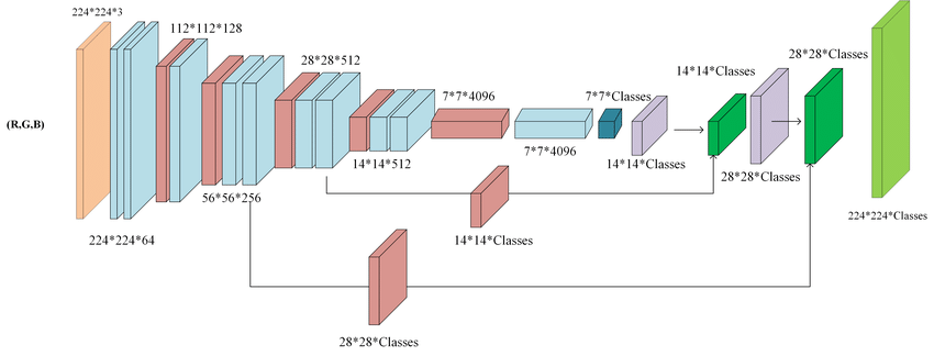
Network Architecture
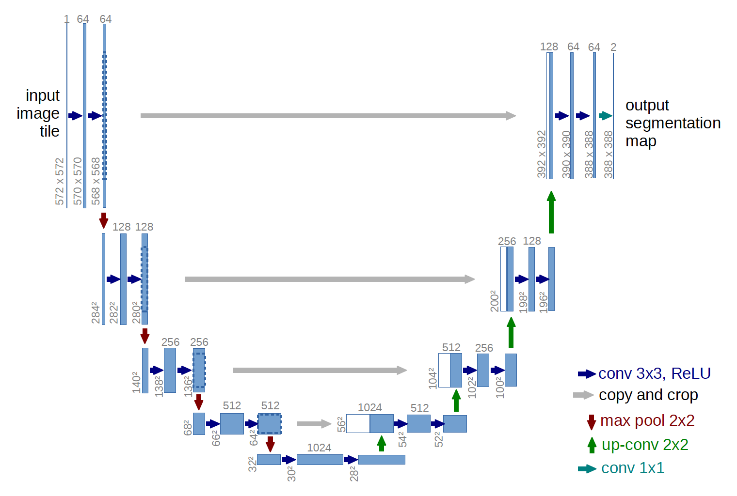
- Contracting Path (left half) - encoder
- repeated $3\times3$ convolutions + ReLU + $2\times2$ max pooling [downsampling]
- VGG based architecture
- downsampling: double the number of feature channels
- convolutions: unpadded
: extract spatial context using convolutions
- repeated $3\times3$ convolutions + ReLU + $2\times2$ max pooling [downsampling]
- Expansive Path (right half) - decoder
- [upsampling] $2\times2$ up-convolution + concat with cropped feature map + $3\times3$ convolutions + ReLU
- upsampling: halve the number of feature channels
- concatenation: skip connection between encoder and decoder → combine context information to localization step to enhance pixel segmentation
- cropping: necessary due to the loss of border pixels in every convolution
- unpadded convolution → different input & output size (572572 & 388388): missing border pixels
- solution 1) mirror extrapolation
- extrapolate the missing context by mirroring the input image instead of zero-padding
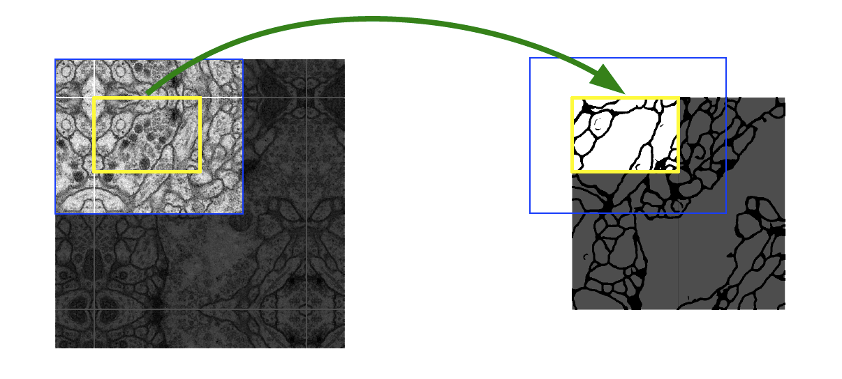
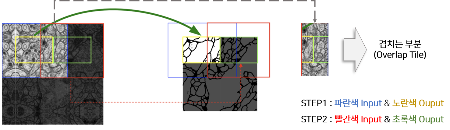
- solution 2) overlap-tile strategy
- generate seamless segmentation that only pixels for which the full context is available from the input image
- important to apply to large images (by separating the original input into overlapping tiles)
- cropping: necessary due to the loss of border pixels in every convolution
: increase localization accuracy by using both upsampled information and context feature map
- final layer
- $1\times1$ convolution: map each component feature vector to number of classes
- classification without FC layer to preserve spatial information
- $1\times1$ convolution: map each component feature vector to number of classes
Training
- implementation: SGD of Caffe
- to minimize overhead: large input tiles over a large batch size → reduce batch to a single image
- loss: pixel-wise soft-max function combined with cross entropy
- pixel-wise soft-max
- $p_k(x):\text{ probability that pixel }x \text{ belongs to class }k$
- $a_k(x): \text{logit that pixel }x \text{ belongs to class }k$ (model output)
- cross entropy loss
- penalize each pixel if $p_{l(x)}(x)$ deviates from 1
- $p_{l(x)}(x) =1 \text{ if pixel }x \text{ belongs to class }l(x)$
- $l(x): \text{GT label of pixel }x$
- penalize each pixel if $p_{l(x)}(x)$ deviates from 1
-
weight map

- large if pixel x is close to the borders → more weight for border adjacent pixels
- $w_0, \sigma: \text{hyperparameters; by defualt: } 10, 5$
- $w_c(x): \text{weight map to balance the class frequencies}$
- more weight to less frequent labels → learn even the segments of small area
- $d_1(x): \text{pixel }x’s \text{ distance to the border of the nearest cell}$
- $d_2(x): \text{pixel }x’s \text{ distance to the border of the second nearest cell}$
- pre-computed weight map for each ground truth segmentation: compensate different frequency of pixels from a certain class in the training sset → force the network to learn small separation borders
- pixel-wise soft-max
-
Why weight loss?
→ proportion of border pixels is low: without weight loss, borders between different objects that belong to the same class might be ignored and displayed as a single object
Experiments
- segmentation of neuronal structures [EM segmentation challenge]
- warping error: segmentation metric, cost function for learning boundary detection
- rand error: defined as 1 - the maximal F-score of the foreground-restricted Rand index, measure of similarity between two clusters or segmentations
- pixel error: squared Euclidean distance between the original and the result labels

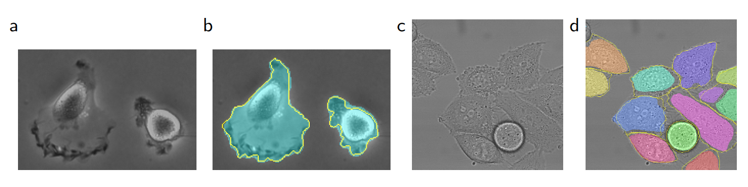
- light microscopic images [ISBI cell tracking challenges]
- IOU results (intersection over union)
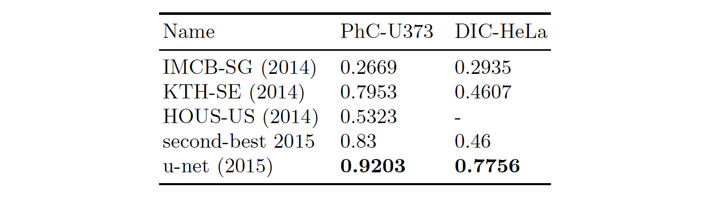
- segmentation results
Contributions
- faster training speed
- optimize trade-off between good localization and the use of context