Noise-contrastive estimation: A new estimation principle for unnormalized statistical models

Michael Gutmann, Aapo Hyvärinen

Proceedings of the Thirteenth International Conference on Artificial Intelligence and Statistics, PMLR 9:297-304, 2010.

http://proceedings.mlr.press/v9/gutmann10a/gutmann10a.pdf

Contribution of NCE

a method to estimate unnormalized parameterized statistical models
provides a theoretical connection between unsupervised and supervised learning

Introduction

Motivation

Ideally, we want to obtain the unknown true data pdf, it’s difficult to get an exact closed-form solution analytically.

Even numerically (with iterative calculations), comparing all individual samples at every iteration is computationally burdensome and wasteful.

ex) Normalization problem (i.e. Issue with using softmax to normalize)

with large number of classes, we have to compute all probabilities and all values in the denominator even though only 1 term lives, as loss depends on every output

→ calculating softmax probabilities can be a waste of computation

→ But we still want to get and utilize information of the true data pdf.

→ Solution: To get information about the true data distribution, we make simplifications and detours to estimate the true data pdf

ex. negative sampling, NCE

~~(근데 estimation도 쉽지 않을 수 있음… so the authors propose NCE. 이 다음 섹션에는 estimation 을 어떻게 하면 좋을지 좀 더 알아보자~)~~

Estimation of parameterized statistical models (i.e. true data pdf)

true data pdf’s are often represented in form of a parameterized model (i.e. use statistical assumptions like $\sim N(\mu, \sigma^2)$) and normalized for convenience (e.g. consider output like probabilities)
but deriving the normalization constant can be difficult
estimation of unnormalized parameterized statistical models → a computationally difficult problem

The basic estimation problem formulation

$\mathbf{x} \in \mathbb{R}^n \sim p_d(.)$ ← an unknown data prob dist’n ftn (pdf)
$p_d(.)$ : modeled by a parameterized family of functions ${ p_m(.; \alpha) }_\alpha$ where $\alpha$ is a vector of parameters
- we assume $p_d(.) \in { p_m(.; \alpha) }_\alpha$ → i.e. $p_d(.) = p_m(.;\alpha^)$ for some parameter $\alpha^$
  
  → issue: how to estimate $\alpha$ from the observed sample by maximizing some objective function

Solution to estimation problem

solution $\hat{\alpha}$ to the estimation problem must yield a properly normalized pdf $p_m(.;\hat{\alpha})$

→ i.e. $\displaystyle \int p_m(\mathbf{u}; \hat{\alpha}) \, d\mathbf{u} = 1$ ⇒ becomes a constraint in the optimization problem
- this constraint can always be fulfilled by redefining estimated pdf as $p_m(.;\alpha)$ $\displaystyle = \frac{p_m^0(.;\alpha)}{Z(\alpha)}$ , where $\displaystyle Z(\alpha) = \int p_m^0(\mathbf{u};\alpha) \, d\mathbf{u}$
- $p_m^0(.;\alpha)$: functional form of the pdf → does not need to integrate to 1
  - functional form: algebraic form of a relationship between a dependent variable and regressors or explanatory variables. (ex. linear, semi-log, double-log, reciprocal… → a concrete example: $d = at^2/2$) → interpretation of coefficients become different depending on the functional form
- $Z(\alpha)$: normalizing constant ← this is the real problem because
  - the integral is rarely analytically tractable (i.e. we don’t usually get a closed-form solution)
  - with high-dim data, numerical integration is difficult
    
    → i.e. it’s difficult to compute probabilities of all elements of the pdf $p_m(.;\alpha)$
  - examples of statistical models where $Z(\alpha)$ is a problem: Markov random fields, energy-based models, multilayer networks
    - Markov Random Field (MRF): a graphical model of a joint pdf → given the grey nodes, black node is not directly connected to the white nodes
      
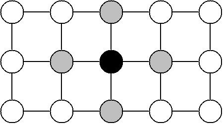
      Given the grey nodes, the black node is conditionally independent of all other nodes.
Approaches to dealing with $Z(\alpha)$
1. consider normalization constant as an additional parameter of the model
  
  → not possible for MLE: likelihood can be made arbitrarily large by making $Z(\alpha) \rightarrow 0$ (i.e. $\frac{\partial l(\alpha)}{\partial \alpha} = \frac{\sum Z(\alpha)}{\sum p_m^0(.;\alpha)} = 0$ 이 되는 $\alpha = \mathrm{MLE}$ 니까 분자를 0으로 보내버리기)
2. estimate the model directly using $p_m^0(.;\alpha)$ without computation of the integral that defines $Z(\alpha)$
  
  → i.e. estimation of unnormalized models
  - ex) contrastive divergence, score matching, … and NCE! (which shows advantages over the previous solutions)
→ NCE: use both approaches 1 and 2
- Both the parameter $\alpha$ in the unnormalized pdf $p_m^0(.;\alpha)$ and the normalization constant can be estimated by maximization of the same objective function.
- basic idea: to estimate the parameters of pdf by learning to discriminate between the data x and some artificially generated noise y by contrasting between x and y.
  
  → hence the name: “noise-contrastive estimation”

Formal definition of NCE

Recall estimated pdf: $\displaystyle p_m(.;\alpha) = \frac{p_m^0(.;\alpha)}{Z(\alpha)}$ , where $Z(\alpha) = \displaystyle \int p_m^0(\mathbf{u};\alpha) \, d\mathbf{u}$

To estimate normalized pdf $p_m(.;\alpha)$ with unnormalized pdf $p_m^0(.;\alpha)$, include the normalization constant as another parameter c of the model

→ $\mathrm{ln} \, p_m(.;\alpha) = \displaystyle \mathrm{ln} \,\frac{p_m^0(.;\alpha)}{Z(\alpha)} = \mathrm{ln} \, p_m^0(.;\alpha) - \mathrm{ln}\,Z(\alpha) = \mathrm{ln} \, p_m^0(.;\alpha) + c$ , where $\theta = {\alpha, c}, \, c =-\mathrm{ln} Z(\alpha)$

→ $p_m(.;\alpha)$ only integrates to 1 for a specific choice of c

observed data set: $X = (\mathbf{x}_1, … , \mathbf{x}_T) \sim p_m(.)$
artificially generated data set of noise $Y = (\mathbf{y}_1, … , \mathbf{y}_T) \sim p_n(.)$ ← known distribution (design parameter that we choose)
want to maximize objective function: $J_T(\theta) = \displaystyle \frac{1}{2T} \sum_t \mathrm{ln} [h(\mathbf{x}_t;\theta)] + \mathrm{ln} [1-h(\mathbf{y}_t;\theta)]$
- where $h(\mathbf{u};\theta) = \displaystyle \frac{1}{1+\mathrm{exp}[-G(\mathbf{u};\theta)]}$ and $G(\mathbf{u};\theta) = \mathrm{ln} \, p_m(\mathbf{u};\theta) - \mathrm{ln} \, p_n(\mathbf{u}) = \displaystyle \mathrm{ln}\frac{ \, p_m(\mathbf{u};\theta)}{p_n(\mathbf{u})}$
- and logistic function is $r(.)$, making $h(\mathbf{u};\theta) = r(G(\mathbf{u};\theta))$
  
  → recall: logistic function $y = \displaystyle \sigma(x) = \frac{1}{1+e^{-x}}$ : $[-\infty, \infty] \rightarrow 0 \sim 1$ (like probability) ⇒ leads to $x = \mathrm{ln}(y) - \mathrm{ln}(1-y)$
  
  → use log-odds ratio (logit) for logistic regression (where input came from one class instead of another): $log(\frac{p_1}{p_2}) = log(\frac{p_1}{1-p_1})$ (input came from true distn $p_m$ instead of noise distn $p_n$): $log(\frac{p_m}{p_n}) = log(p_m) - log(p_n)$
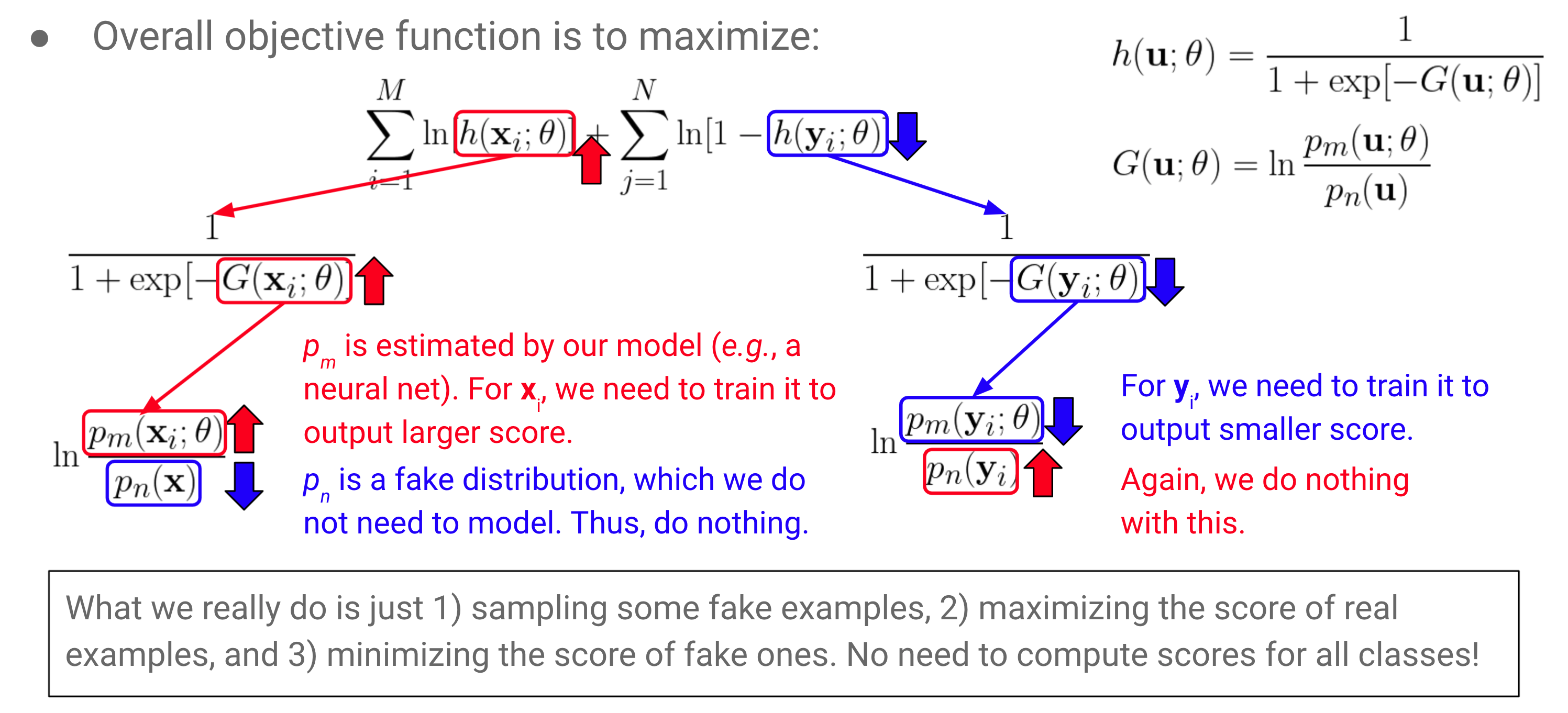
from 21-1 MLVU Lecture 15, slide 50 ⇒ p_n(x), p_n(y_i) 는 우리가 알고 있는 분포에서 얻을 수 있으니까 irrelevant to the learning process

Fundamental statistical properties: asymptotic behavior of $\hat{\theta}_T$

as sample size T↑, due to weak law of large numbers (WLLN), objective function becomes:

\[\begin{aligned} J_T(\theta) = \displaystyle \frac{1}{2T} \sum_t \mathrm{ln} [h(\mathbf{x}_t;\theta)] + \mathrm{ln} [1-h(\mathbf{y}_t;\theta)] \, \xrightarrow{p} J(\theta) & = \displaystyle \frac{1}{2} E \,\mathrm{ln} [h(\mathbf{x};\theta)] + \mathrm{ln} [1-h(\mathbf{y};\theta)] \\ \xrightarrow{f(.) = \mathrm{ln} \, p_m(.;\theta)} \tilde{J}(f) & = \displaystyle \frac{1}{2} E \,\mathrm{ln} [ r\{f(\mathbf{x} - \mathrm{ln}\,p_n(\mathbf{x})\} ] + \mathrm{ln} [1-r\{f(\mathbf{x} - \mathrm{ln}\,p_n(\mathbf{x})\}] \end{aligned}\]

ref) WLLN, convergence in probability ($\xrightarrow{p}$)

ref) weak law of large numbers: sample average converges in probability towards expected value

→ $\bar{X}n \xrightarrow{p} \mu$ when $n \rightarrow \infty$. i.e. $\displaystyle \lim{n \rightarrow \infty} Pr(

\bar{X}_n - \mu

> \epsilon) = 0, \,\, \forall \epsilon >0$

ref) convergence in probability: sequence ${X_n} \xrightarrow{p}$ r.v. $X \Leftrightarrow \displaystyle \lim_{n \rightarrow \infty} Pr(

X_n - X

> \epsilon) = 0, \,\, \forall \epsilon >0$

→ probability of an ‘unusual’ outcome becomes smaller and smaller as the sequence progresses

→ converge in probability ⇒ estimator is consistent

data pdf $p_d(.)$ can be found by maximization of $\tilde{J}$ by learning a classifier under the ideal situation of infinite amount of data:

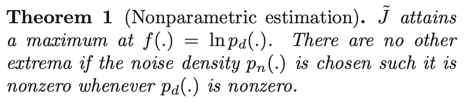
similar behavior of $\tilde{J}$ and data pdf $p_d(.)$
no need for normalizing constraint for f(.) when performing maximization
- b/c maximizing pdf is found to have unit integral automatically
- cf) constraint for MLE: exp(f) must integrate to 1

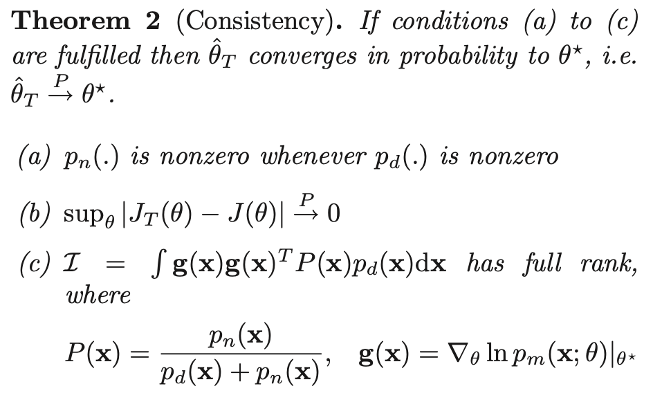
$\hat{\theta}_T$ ($\theta$ that globally maximizes $J_T$) converges to $\theta^*$
thus, leads to correct estimate of $p_d(.)$ as sample size T increases
log-normalization constant is part of parameters for unnormalized models → maximizing obj ftn leads to correct estimates for both $\alpha$ and c
- cf) not possible with likelihood

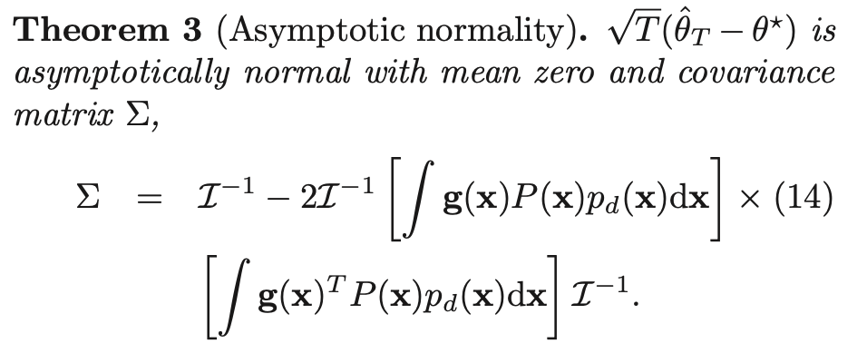
$\sqrt{T} (\hat{\theta}_T - \theta^*) \sim N(0, \Sigma)$

trace of covariance matrix: sometimes referred to as total/overall variation of the random variable

→ informal measure of ‘spread’

→ NCE can be generalized in a statistically nice form (i.e. based on normal distribution) to large sample sizes

Choosing the appropriate contrastive noise distribution

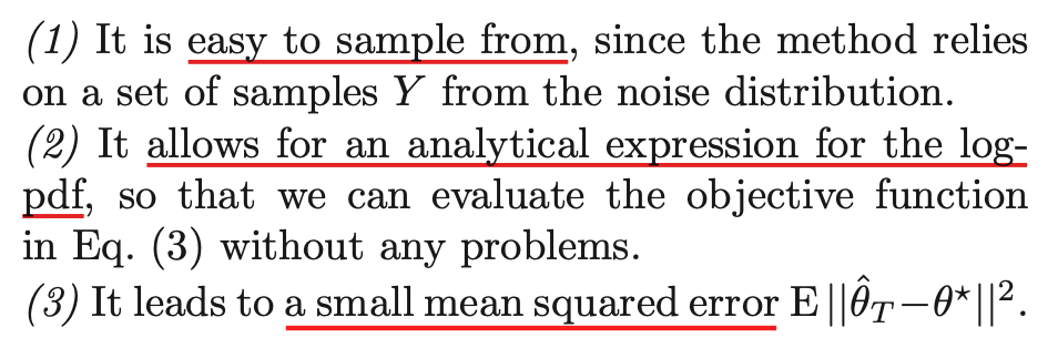
noise distribution $p_n(.)$ is a design parameter
ideal properties of $p_n(.)$:

→ objective function in Eq. (3):

$J_T(\theta) = \displaystyle \frac{1}{2T} \sum_t \mathrm{ln} [h(\mathbf{x}_t;\theta)] + \mathrm{ln} [1-h(\mathbf{y}_t;\theta)]$

In practice: Gaussian or uniform distribution, a Gaussian mixture distribution, or an ICA distribution → satisfies (1), (2)
try to have $p_n(.) \approx p_m(.)$, or else learning will be too easy (similar approach to semi-hard/smart negative mining?)
- if $p_n(.) = p_m(.)$, [$\Sigma$ in Thm 3] == 2*[Cramér-Rao bound] → MSE is closer to theoretical optimum
- ref) Details on Cramér-Rao Bound
  
  Cramér-Rao bound (CRB): a lower bound on the variance of unbiased estimators of a deterministic (fixed, though unknown) parameter
  - var(any unbiased estimator) ≥ inverse(Fisher information): $Var(\hat{\theta}) \geq \frac{1}{I(\theta)}$ : theoretically, variance cannot be lower than $\frac{1}{I(\theta)}$
    
    ref) Fisher Information $I(\theta)$: a way of measuring the amount of information that an observable random variable X carries about an unknown parameter $\theta$ of a distribution that models X
    - if P(event) is small, occurrence of this event gives us lots of information
    - for true $\theta$, likelihood ↑ (i.e. derivative of log-likelihood → 0)
      
      ⇒ an r.v. $\hat{\theta}$ $\approx \theta$ does not provide much information about $\theta$ ⇒ $I(\hat{\theta}) \downarrow$
  - unbiased estimators that satisfy CRB and have variance that equals $\frac{1}{I(\theta)}$ are fully efficient
    
    (i.e. have the lowest possible MSE among all unbiased estimators ⇒ Minimum Variance Unbiased estimator (MVUE))
    
    → the paper probably means: if parameters of $p_n(.) = p_m(.)$, [$\Sigma$ in Thm 3] == 2*$[ \frac{1}{I(\theta)} ]$ because “estimator converges in probability ⇒ estimator is asymptotically consistent” (with sufficiently large T, variance should be minimal)
  - the precision to which we can estimate $\theta$ is fundamentally limited by the Fisher information of the likelihood function.

Connection to supervised learning

with NCE, an unsupervised task of learning the data distribution P

→ has become a supervised Log Reg problem for classification (with labels indicating if a word is the true target or from the noise distribution)

objective function $J_T(\theta)$ can also be derived in supervised learning setting

→ log-likelihood in a logistic regression model that discriminates observed data $X$ from noise $Y$

$U = (\mathbf{u}_1, … , \mathbf{u}_{2T})$ → $X \cup Y$
each data point $\mathbf{u}_t$ has a binary class label $C_t: C_t = \begin{cases}1 \,\, (\mathbf{u}_t \in X)\\ 0 \,\, (\mathbf{u}_t \in Y)\end{cases}$

in logistic regression, posterior probabilities of classes given the data $\mathbf{u}_t$ are estimated

→ as pdf $p_d(.)$ of data $\mathbf{x}$ is unknown (i.e. we need to find parameters $\theta = {\alpha, c}$), class-conditional probability $p(.

C=1)$ is modeled with $p_m(.;\theta)^2$

→ class-conditional pdf’s become: $\begin{cases} p(\mathbf{u}|C=1;\theta) = p_m(\mathbf{u};\theta) \\ p(\mathbf{u}|C=0) = p_n(\mathbf{u}) \end{cases}$

Since each class labels have uniform prior probabilities (i.e. P(C=1) = P(C=0) = 1/2),

→ posterior probabilities become: $\begin{cases} \begin{aligned} P(C=1|\mathbf{u};\theta) & = \displaystyle \frac{p_m(\mathbf{u};\theta)}{p_m(\mathbf{u};\theta)+p_n(\mathbf{u})} \\ & = h(\mathbf{u};\theta) \\ P(C=0|\mathbf{u};\theta) & = 1-h(\mathbf{u};\theta) \end{aligned} \end{cases}$

Details on calculations

posterior probability = the updated probability of an event after considering the new information

→ calculated by updating the prior probability using Bayes’ theorem $P(A

B) = \displaystyle \frac{P(A \cap B)}{P(B)} = \frac{P(A)P(B

A)}{P(B)}$

→ statistically, prior probability = P(A), P(B), and posterior probability = P(A

in this case,

prior probabilities = P(C=1) = P(C=0) = 1/2
posterior probabilities = $\begin{cases} \begin{aligned} \displaystyle P(C=1|\mathbf{u};\theta) & = \frac{P(C=1 \cap \mathbf{u} ;\theta)}{P(\mathbf{u};\theta)} = \frac{P(C=1) P(\mathbf{u} | C=1; \theta)}{P(\mathbf{u};\theta)} = \frac{\frac{1}{2} p_m(\mathbf{u};\theta)}{\frac{1}{2} p_m(\mathbf{u};\theta)+\frac{1}{2} p_n(\mathbf{u})} \

& = \frac{p_m(\mathbf{u};\theta)}{p_m(\mathbf{u};\theta)+p_n(\mathbf{u})} = \frac{1}{\frac{p_m(\mathbf{u};\theta) + p_n(\mathbf{u})}{p_m(\mathbf{u};\theta)}} = \frac{1}{1+ \frac{ p_n(\mathbf{u})}{p_m(\mathbf{u};\theta)}} = \frac{1}{1+ \mathrm{exp}[\mathrm{ln}\frac{ p_n(\mathbf{u})}{p_m(\mathbf{u};\theta)} ] } = \frac{1}{1+ \mathrm{exp}[-G(\mathbf{u};\theta)] } \

& = h(\mathbf{u};\theta) \

P(C=0|\mathbf{u};\theta) & = \frac{P(C=0 \cap \mathbf{u} ;\theta)}{P(\mathbf{u};\theta)} = \frac{P(C=0) P(\mathbf{u} | C=0)}{P(\mathbf{u};\theta)} = \frac{\frac{1}{2} p_n(\mathbf{u})}{\frac{1}{2} p_m(\mathbf{u};\theta)+\frac{1}{2} p_n(\mathbf{u})} \

& = \frac{p_n(\mathbf{u})}{p_m(\mathbf{u};\theta)+p_n(\mathbf{u})} \

& = 1-h(\mathbf{u};\theta) \end{aligned} \end{cases}$

→ Note: we write $\theta$ only when applicable in the equations above (i.e. when we need to consider parameters $\theta = {\alpha, c}$

class labels $C_t \sim Bernoulli(.)$, so log-likelihood of $\theta$ becomes:

\[\begin{aligned} l(\theta) & = \displaystyle \sum_t \mathrm{ln} P(C_t = 1 | \mathbf{u}; \theta) + (1-C_t)\mathrm{ln} P(C_t = 0 | \mathbf{u}; \theta) \\ & = \sum_t \mathrm{ln} [h(\mathbf{x}_t;\theta)] + \mathrm{ln} [1-h(\mathbf{y}_t;\theta)] \end{aligned}\]

→ same as the objective function for NCE!

Simulations & Comparisons

Estimation of ICA model using NCE

ICA: Independent component analysis

noise y ~ Gaussian with same mean and covariance matrix as x
data $\mathbf{x} \in \mathbb{R}^4$ generated via ICA model $\mathbf{x} = A \mathbf{s}$ , where mixing matrix $A = (\mathbf{a}_1, … \mathbf{a}_4), \, s \sim$ Laplace(0, 1) (i.e. Double Exponential (DE))
parameters $\theta$ estimated by learning to discriminate between data x and noise y (i.e. by maximizing objective function $J_T$)
optimization via conjugate gradient algorithm

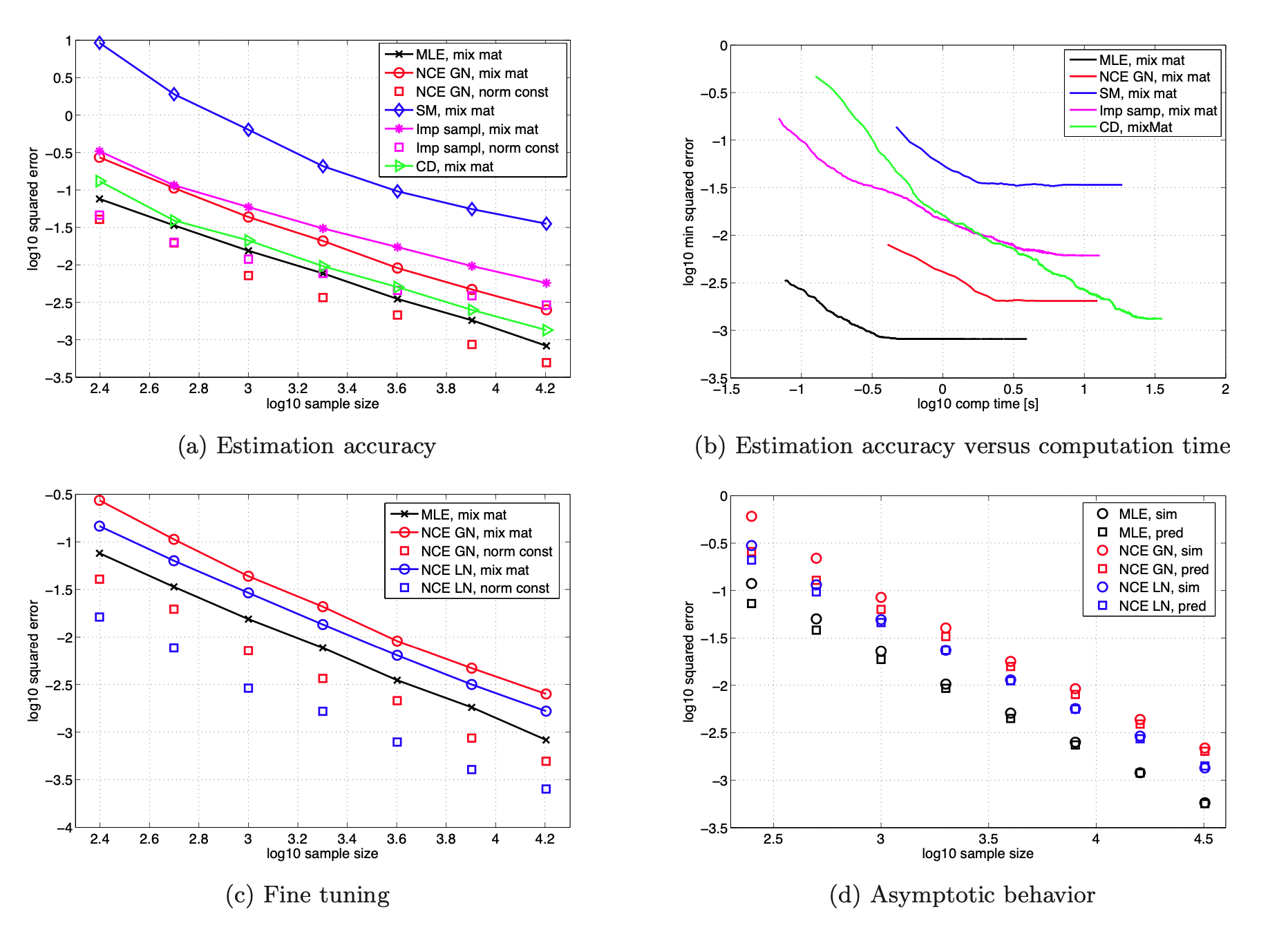
Comparison of performance to other estimation methods

Methods compared: NCE, MLE (reference), contrastive divergence (CD), score matching (SM)

Fig (a): MSE $\mathrm{E} \hat{\theta}_T - \theta^* ^2$
- performance: NCE (with normalizing constant) > MLE (normalizing constant calculated with importance sampling) > CD (for fixed sample sizes) > SM
- NCE: MSE for demixing matrix and log-normalization constant c decreases as sample size T increases → estimator is consistent
- NCE > MLE: estimate of c is more accurate
- CD: var(squared error) was very high (almost 50x higher than NCE…)
Fig (b): tradeoff between statistical and computational efficiency
- MLE: shortest computation time → works well with properly normalized pdf’s
- NCE: (among methods for unnormalized models) required least computation time → 3x faster than CD
Fig (c): confirming $p_n(.) \approx p_m(.)$ yields smaller MSE (statistically significant)
- NCE: Laplacian contrastive noise gave better estimates than Gaussian noise (recall: data x was generated with s~Laplace(0,1))

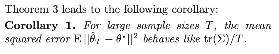
Fig (d): confirm behaviors of $\mathrm{E}

\hat{\theta}_T - \theta^*

^2 \approx \mathrm{tr}(\Sigma)/T$ for large sample sizes T (Corollary 1)

Simulations with natural images

application of NCE on learning of an energy-based two-layer model and a Markov random field model of natural images

Patch model
- input: 30 x 30 pixel patches from wild-life scene images + 4 preprocessing steps:
  - removed DC component of each patch
  - whitened: normalization + decorrelation
  - dim reduction: 900 → 225
  - normalize each patch to have zero DV value and unit variance
    
    → whitened data projected onto a sphere
- noise ~ uniform distribution on sphere
- output: NCE (pooling patterns) of models for natural images
Markov random field
- same data + preprocessing + contrastive noise as patch model
- input: 45 x 45 pixel patches
- output: NCE (learned filters) of models for natural images

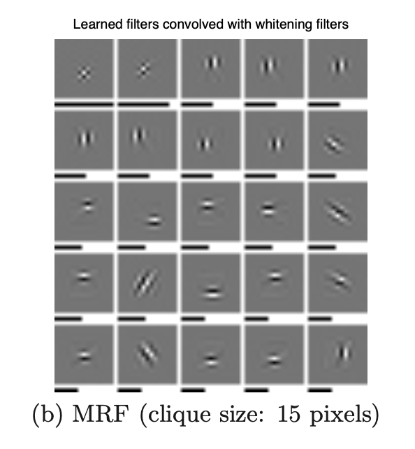
→ NCE can successfully estimate a large-scale two-layer model and a Markov random field

→ confirmed validity of the estimation principle using NCE

Negative Sampling vs. NCE

Recap of Motivation

Ideally, we want to obtain the unknown true data pdf, it’s difficult to get an exact closed-form solution analytically.

Even numerically (with iterative calculations), comparing all individual samples at every iteration is computationally burdensome and wasteful.

ex) Normalization problem (i.e. Issue with using softmax to normalize)

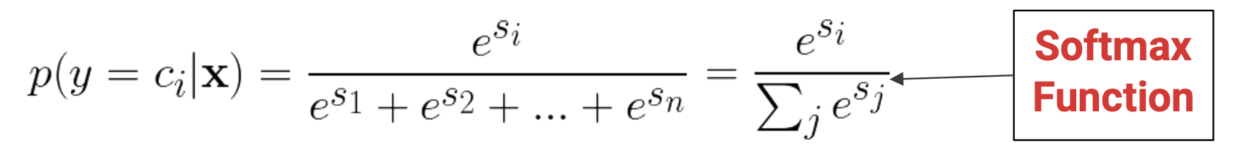
with large number of classes, we have to compute all probabilities and all values in the denominator even though only 1 term lives, as loss depends on every output

→ calculating softmax probabilities can be a waste of computation

→ But we still want to get and utilize information of the true data pdf.

Solutions: Negative Sampling vs. NCE

To get information about the true data distribution, we make simplifications and detours to approximate/estimate the true data pdf!

By discriminating, or comparing, between data and noise → we learn properties of the data in the form of a statistical model

→ “learning by comparison”

1. Negative sampling:

get true pdf info indirectly
by comparing real labels vs. noise labels
- label for GT is 1 for true target word, and 0 for random samples of the incorrect target words
of sampled noise/negative data **to get a good approximation of the loss

→still satisfies our objective to ↑prob for positive pair and obtain information about the positive data distribution
~~Example of study that used negative sampling: simCLR~~

2. NCE (Noise Contrastive Estimator):

similar implementation with negative sampling as you “contrast with the noise to get your estimation”, 근데 이제 이론적 배경을 곁들인…

get (true) pdf info directly
by comparing data distribution vs. noise distribution (i.e. compare the parameters $\theta$ of distributions)
- use log-odds ratio (logit) for logistic regression (where input came from one class instead of another): $log(\frac{p_1}{p_2}) = log(\frac{p_1}{1-p_1})$ → (input came from true distn P instead of noise distn Q): $log(\frac{P}{Q}) = log(P) - log(Q)$
with reference to the known noise distribution
we don’t know P, but we can set Q to be whatever we want → makes calculating log(Q) straightforward (we can analytically calculate any particular word’s probability according to dist’n Q)

→ unsupervised task of learning the data distribution P has become a supervised Log Reg problem (with labels indicating if a word is the true target or from the noise distribution)

→ so, NCE 는 data pdf에 대한 정보를 얻는 과정에서 negative sampling 보다 이론적으로 더 탄탄한/general framework

Theoretical comparison

NCE and negative sampling have different definitions of conditional probability

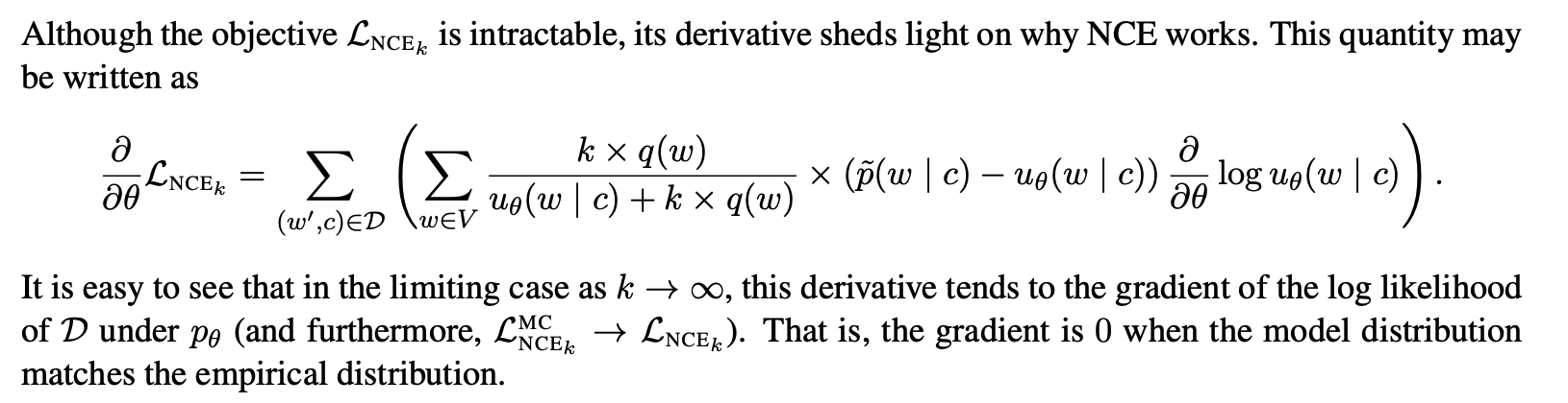
given a general language model: predict word w in vocabulary V based on given context c, where $u_\theta(w,c) = e^{s_\theta(w,c)}$ and $Z(c)$ is normalizing constant

$\displaystyle p_\theta (w|c) = \frac{u_\theta(w,c)}{\sum_{w’ \in V} u_\theta(w’,c)} = \frac{u_\theta(w,c)}{Z_\theta (c)} \,\,… \,\,(1)$
conditional probabilities (with class labels D, noise distribution q(w), k noise samples from q):

NCE: $$\begin{cases} \displaystyle p(D=0 | c,w) = \frac{k \times q(w)}{u_\theta(w,c) + k \times q(w)} \

\displaystyle p(D=1 | c,w) = \frac{u_\theta(w,c)}{u_\theta(w,c) + k \times q(w)} \end{cases}$ negative sampling: $\begin{cases} \displaystyle p(D=0 | c,w) = \frac{1}{u_\theta(w,c) + 1} \

\displaystyle p(D=1 | c,w) = \frac{u_\theta(w,c)}{u_\theta(w,c) +1} \end{cases}$$

→ negative sampling == NCE when $k = |V|$ and $q \sim Unif(.)$ ⇒ negative sampling $\sub$ NCE

Summary

NCE: a general parameter estimation technique that is asymptotically unbiased

→ can get solution for (1)
negative sampling: best understood as a family of binary classification models that are useful for learning word representations but not as a general-purpose estimator

→ does not guarantee asymptotic consistency